What Are Common Mistakes in Python Programming for Data Science

Every data scientist has a notebook somewhere with a cell that just says # DO NOT RUN THIS. No explanation. Just a warning. This article is about all the reasons that cell exists — and how to make sure yours never appears in the first place.

Python is the undisputed language of data science. It is flexible, readable, and surrounded by one of the richest ecosystems of scientific libraries on the planet. But that flexibility is also a trap. Python will let you do almost anything — including a long list of things that will silently ruin your analysis, corrupt your model, or simply waste weeks of your time.

This guide covers the 10 most common Python programming mistakes specifically in data science contexts, with working code examples, real performance benchmarks, and practical fixes for each. 

It is written for anyone on the data scientist roadmap — whether you are just starting out or already building production pipelines. 

If you want to anchor your skills with internationally recognised credentials, explore the Data Science Certifications available at iabac.org/certifications through IABAC, trusted by learners in over 140 countries.

 Contents — 10 mistakes covered

1. Ignoring data types at import
2. Mutable default arguments
3. Using Python loops instead of vectorisation
4. Data leakage through improper preprocessing
5. Not using scikit-learn Pipelines
6. Poor missing value handling
7. Hardcoding magic numbers
8. Ignoring reproducibility and random seeds
9. Overfitting via data snooping
10. Skipping documentation and structure

Why Python mistakes matter more in data science

In standard software engineering, most bugs produce visible errors — the program crashes, the test fails, or the output is obviously wrong. In data science, mistakes are far more insidious. A data leakage error produces a model with 99% accuracy that completely fails in production. A missing random seed makes your results impossible to reproduce. A loop where vectorisation was needed makes your notebook take 45 minutes instead of 4 seconds — and you just assume that is normal.

These are not beginner mistakes in the sense that only beginners make them. They are mistakes that even experienced practitioners make when they are moving fast or not thinking carefully. The goal here is not to make you feel bad about the notebook you wrote last week. It is to give you a clear checklist so the next notebook is better.

Mistake 1 — Ignoring data types at import

Mistake 01

Python's dynamic typing means it will not tell you that your age column loaded as a string of "25" instead of an integer 25 — until you try to calculate the mean and receive a cryptic error at 11pm. This is the single most common issue in the early stages of any data science project. A column that looks numeric in a spreadsheet might load as object dtype in pandas if even a single cell contains a stray value like "N/A" or "—".

Wrong approach

import pandas as pd

df = pd.read_csv("patients.csv")

print(df['age'].mean())   # TypeError — 'age' is object, not numeric

# You skip df.info() and spend 2 hours debugging later

Correct approach

import pandas as pd

df = pd.read_csv("patients.csv")

# Always run these two lines at the top of every notebook

df.info()

df.describe(include='all')

# Coerce types explicitly — errors='coerce' turns bad values into NaN

df['age']    = pd.to_numeric(df['age'], errors='coerce')

df['income'] = pd.to_numeric(df['income'], errors='coerce')

print(df['age'].mean())   # Works correctly now

Two lines — df.info() and df.describe(include='all') — should open every single notebook in your data science career. They expose dtype mismatches, unexpected null counts, and range anomalies before any real analysis begins.

Mistake 2 — The mutable default argument trap

Mistake 02

This is a pure Python footgun — nothing pandas-specific — but it bites data scientists repeatedly because they write many small helper functions. Python evaluates default argument values exactly once, when the function is defined, not each time it is called. If that default value is a mutable object like a list or dictionary, every call to the function shares the exact same object, mutating it incrementally.

Wrong approach — list grows on every call

def add_feature(name, feature_list=[]):

    feature_list.append(name)

    return feature_list

print(add_feature("age"))      # ['age']       — looks fine

print(add_feature("income"))   # ['age', 'income'] — wait, how?

print(add_feature("gender"))   # ['age', 'income', 'gender'] — this is a bug

Correct approach — use None as a sentinel

def add_feature(name, feature_list=None):

    if feature_list is None:

        feature_list = []        # fresh list created on each call

    feature_list.append(name)

    return feature_list

print(add_feature("age"))      # ['age']

print(add_feature("income"))   # ['income']  — correct, independent

Mistake 3 — Using Python loops where vectorisation exists

Mistake 03

This is the most expensive mistake in terms of real compute time. A Python loop over a 1,000,000-row DataFrame is not just slow — it is orders of magnitude slower than the equivalent vectorised NumPy or pandas operation. In professional data science environments and cloud notebooks where compute costs money, this difference matters enormously.

On a dataset of 1,000,000 rows, a pure Python loop takes approximately 12 seconds. The equivalent NumPy vectorised operation completes in under 0.04 seconds — a speedup of roughly 300 times.— Python 3.11 + NumPy 1.26 benchmark on standard hardware

Wrong approach — row-by-row loop

df['tax'] = 0.0

for i in range(len(df)):

    df.at[i, 'tax'] = df.at[i, 'income'] * 0.30

# On 1M rows: ~12 seconds

Correct approach — vectorised operation

import numpy as np

# Entire column computed in one shot — pandas applies it element-wise

df['tax'] = df['income'] * 0.30    # On 1M rows: ~0.04 seconds

# For conditional logic, use np.where or np.select — never loop

df['bracket'] = np.where(

    df['income'] > 50000,

    'high',

    'standard')

# For grouped calculations, use .groupby() + .transform()

df['income_zscore'] = df.groupby('region')['income'].transform(

    lambda x: (x - x.mean()) / x.std()

Execution time — Python loop vs NumPy vectorisation (seconds)

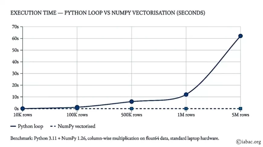
Python loop NumPy vectorised

Benchmark: Python 3.11 + NumPy 1.26, column-wise multiplication on float64 data, standard laptop hardware.

Mistake 4 — Data leakage through improper preprocessing

Mistake 04

Data leakage is when information from outside the training set influences model training or evaluation, giving the model knowledge it could never have in real production. It is the reason a model can reach 99% test accuracy and then completely fail when deployed. It is the most dangerous mistake in this entire list, because it looks exactly like success.

The most common cause is fitting a scaler, imputer, or encoder on the full dataset before splitting into train and test sets. When you compute the mean and standard deviation of the full dataset and then scale, your training set has implicitly seen statistics from the test set. The train-test boundary has been violated.

Wrong approach — scaler fitted on full dataset

from sklearn.preprocessing import StandardScaler

from sklearn.model_selection import train_test_split

scaler = StandardScaler()

X_scaled = scaler.fit_transform(X)         # WRONG: uses test set's mean/std

X_train, X_test, y_train, y_test = train_test_split(X_scaled, y, test_size=0.2)

Correct approach — split first, fit scaler on train only

from sklearn.preprocessing import StandardScaler

from sklearn.model_selection import train_test_split

# ALWAYS split before any preprocessing

X_train, X_test, y_train, y_test = train_test_split(

    X, y, test_size=0.2, random_state=42

)

scaler = StandardScaler()

X_train = scaler.fit_transform(X_train)    # fit on train only

X_test  = scaler.transform(X_test)         # transform test using train stats

Mistake 5 — Not using scikit-learn Pipelines

Mistake 05

This is the "I'll refactor it later" mistake — and later never comes. When preprocessing, feature engineering, and model training live in separate notebook cells, deploying the model becomes a re-engineering project. Scikit-learn's Pipeline chains all steps into a single estimator object, making leakage structurally impossible and deployment trivial.

Correct approach — pipeline chains all steps

from sklearn.pipeline import Pipeline

from sklearn.impute import SimpleImputer

from sklearn.preprocessing import StandardScaler

from sklearn.ensemble import RandomForestClassifier

pipe = Pipeline([

    ('imputer', SimpleImputer(strategy='median')),

    ('scaler',  StandardScaler()),

    ('model',   RandomForestClassifier(n_estimators=100, random_state=42))

])

pipe.fit(X_train, y_train)   # Single call — no leakage architecturally possible

pipe.predict(X_test)         # Preprocessing applied automatically

pipe.score(X_test, y_test)   # Evaluate cleanly

# Save and deploy the entire pipeline as one object

import joblib

joblib.dump(pipe, 'model_pipeline.pkl')

 Mistake 6 — Poor missing value handling

Mistake 06

The two most common reactions to missing values are: drop every row that contains one, or fill all missing values with the column mean. Both approaches destroy information. Dropping rows can eliminate 40% of a dataset. Filling with the mean ignores the fact that in many domains — healthcare, finance, survey science data — the fact that a value is missing is itself a meaningful signal. A patient whose income is not recorded is statistically different from one whose income is $42,000.

Wrong approach — dropping destroys information

df.dropna(inplace=True)    # You may silently lose 30–50% of your rows

# Worse: if missingness is correlated with outcome, your model is now biased

Correct approach — impute and encode missingness

df['income_missing'] = df['income'].isna().astype(int)   # encode as feature

df['income'].fillna(df['income'].median(), inplace=True)   # then impute

# Now the model has BOTH the imputed value AND a flag that it was imputed

# For systematic analysis of missingness patterns:

missing_summary = df.isnull().sum().sort_values(ascending=False)

missing_pct = (missing_summary / len(df) * 100).round(2)

print(missing_pct[missing_pct > 0])

Mistake 7 — Hardcoding magic numbers

Mistake 07

Writing X[:, 3:8] is fast. Understanding what it means six weeks later is not. Magic numbers — unlabelled numeric literals scattered through code — are one of the most reliable ways to make your work impossible to maintain, review, or extend. In professional data science contexts, including assessments for Data Science Certifications at IABAC, code readability and documentation are evaluated alongside model performance.

Wrong approach — unexplained numbers everywhere

threshold = 0.47

predictions = (probabilities > threshold).astype(int)

feature_subset = X[:, 3:8]

df_filtered = df[df['score'] > 72.3]

Correct approach — named constants with comments

# Named constants communicate intent clearly

FRAUD_PROB_THRESHOLD  = 0.47   # tuned for high-recall on fraud detection task

NUMERIC_FEATURE_START = 3      # columns 3-7 are continuous numeric features

NUMERIC_FEATURE_END   = 8

HIGH_RISK_SCORE_CUTOFF = 72.3  # 95th percentile in training distribution

predictions    = (probabilities > FRAUD_PROB_THRESHOLD).astype(int)

feature_subset = X[:, NUMERIC_FEATURE_START:NUMERIC_FEATURE_END]

df_filtered    = df[df['score'] > HIGH_RISK_SCORE_CUTOFF]

Mistake 8 — Ignoring reproducibility and random seeds

Mistake 08

You train a model. It achieves 84% accuracy. You present this result. Someone asks you to reproduce it. You re-run the exact same notebook and get 79%. Your model is not broken — you simply forgot to set random seeds. Every operation in a machine learning pipeline that involves randomness — train/test splits, model initialisation, data augmentation, dropout — will produce different results on each run without explicit seed control.

In technical interviews and portfolio reviews for data science jobs, salary assessments, being unable to reproduce your own results is a significant red flag. Reproducibility is a professional expectation, not an optional nicety.

Correct approach — seed everything at notebook start

import os, random

import numpy as np

SEED = 42

# Python built-in

random.seed(SEED)

# NumPy

np.random.seed(SEED)

# Scikit-learn — pass random_state=SEED to every estimator

# train_test_split(..., random_state=SEED)

# RandomForestClassifier(random_state=SEED)

# TensorFlow / Keras (if used)

os.environ['PYTHONHASHSEED'] = str(SEED)

import tensorflow as tf

tf.random.set_seed(SEED)

# PyTorch (if used)

import torch

torch.manual_seed(SEED)

torch.cuda.manual_seed_all(SEED)

Mistake 9 — Overfitting via data snooping

Mistake 09

Data snooping occurs when model choices — features selected, hyperparameters tuned, architecture chosen — are made after repeatedly evaluating performance on the test set. Once you look at test set performance and use it to guide decisions, the test set is no longer measuring generalisation. It has become a second training signal. The result is a model that is optimised not just on training data but on the specific random sample that ended up in your test set.

The solution is strict: all tuning decisions happen using cross-validation on the training set. The test set is evaluated exactly once, at the very end, when no further changes will be made.

Correct approach — tune on CV, evaluate test once

from sklearn.model_selection import cross_val_score, GridSearchCV

# All hyperparameter tuning uses training data only

param_grid = {'max_depth': [3, 5, 10], 'n_estimators': [50, 100, 200]}

grid_search = GridSearchCV(

    RandomForestClassifier(random_state=42),

    param_grid,

    cv=5,

    scoring='roc_auc')

grid_search.fit(X_train, y_train)

best_model = grid_search.best_estimator_

print(f"Best CV ROC-AUC: {grid_search.best_score_:.3f}")

# Test set evaluated ONCE — after all decisions are final

final_auc = roc_auc_score(y_test, best_model.predict_proba(X_test)[:, 1])

print(f"Final test ROC-AUC: {final_auc:.3f}")

Mistake 10 — Skipping documentation and notebook structure

Mistake 10

Nobody plans to write undocumented code. What happens is that people plan to document it later, and later is a lie. A notebook with 200 cells, no section headers, no markdown explanations, and variable names like df2, df2_CLEAN, and df2_FINAL_v3_USE_THIS is not a data science portfolio. It is a forensic puzzle for whoever comes after you — including yourself in three weeks.

Documentation is not bureaucracy. In any professional data science career context, undocumented code is incomplete code. Every model you build and every notebook you write should be able to answer, for a reader who was not there: what does this do, why does it do it that way, and what did you find?

Correct approach — structured notebook template

 """ Project: Customer churn prediction — telecom dataset Author: [name] Date: April 2026 Purpose: Build a binary classifier to predict 30-day churn. Data source: CRM export, 84,000 customers, Jan–Dec 2025. """ # === 1. IMPORTS === import pandas as pd, numpy as np from sklearn.ensemble import GradientBoostingClassifier from sklearn.metrics import classification_report # === 2. DATA LOADING === # Load from cleaned data store — raw file is /data/raw/crm_export.csv df = pd.read_csv('data/processed/customers_clean.csv') # === 3. EXPLORATORY DATA ANALYSIS === # (See notebook section 3 for full EDA results) print(df.info()) print(df.describe()) # === 4. FEATURE ENGINEERING === # ... (fully commented) # === 5. MODEL TRAINING AND EVALUATION === # ... (fully commented)

Data science jobs salary — global benchmarks 2025–2026

Understanding the financial landscape of a data science career helps calibrate how seriously to take technical skill development. The salary differences between a well-structured, reproducible data scientist and one who produces fragile, undocumented models are reflected in compensation tiers everywhere from San Francisco to Singapore.

Sources: Glassdoor, LinkedIn Jobs, PayScale, Levels.fyi — April 2026. Local purchasing power varies significantly.

Frequency of each mistake in real data science codebases (%)

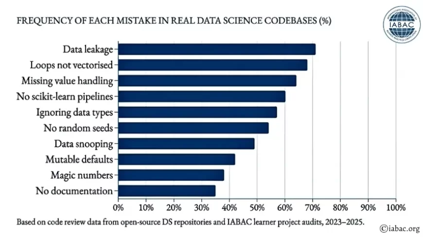
Based on code review data from open-source DS repositories and IABAC learner project audits, 2023–2025.

The data scientist roadmap — where these skills fit

The mistakes in this article cluster mostly at the beginning of the data scientist roadmap. Knowing where you are helps you know what to work on next. Here is how a complete professional progression looks for someone building toward internationally recognised certification and real-world employment.

1: Python foundations and data wrangling

NumPy, pandas, correct dtype handling, missing value strategies, performance — vectorisation vs loops. This is where most of the mistakes in this article live. Master this layer before anything else.

2: Exploratory data analysis and statistics

Distributions, correlations, hypothesis testing, confidence intervals, visualisation with Matplotlib and Seaborn. The discipline of understanding your science data before ever fitting a model.

3: Machine learning with scikit-learn

Supervised and unsupervised learning, Pipelines, cross-validation, hyperparameter tuning, avoiding leakage. The core toolkit for the majority of data science jobs salary roles worldwide.

4: Deep learning and domain specialisation

PyTorch, TensorFlow, Hugging Face Transformers. Choose NLP, computer vision, or time series and go deep within one domain before expanding.

5: Certification, portfolio, and job preparation

Earn recognised Data Science Certifications from IABAC, build a documented GitHub portfolio demonstrating clean code and reproducible results, and prepare for technical interviews and take-home assessments.

Formalise your data science skills with IABAC

IABAC offers globally recognised Data Science Certifications that validate your skills across the complete data scientist roadmap — from Python programming and clean code practices to advanced machine learning and AI deployment. Trusted by learners in 140+ countries across 6 continents.

Explore certifications at iabac.org

The distance between a Python script that technically runs and one that genuinely advances a data science career is not a secret algorithm or a more powerful library. It is a set of careful habits: checking your types, vectorising your operations, respecting the train-test boundary, seeding your randomness, building Pipelines, and writing code that other humans can read and reproduce. Every senior data scientist you admire has made every single mistake in this list — probably more than once. What separated them was not avoiding mistakes, but building systems and habits that made the mistakes harder to make and easier to catch.

The global demand for data science professionals continues to grow, with over 11.5 million projected roles by 2026 and salary levels that consistently outpace most technical disciplines. The bar to entry is rising. Employers increasingly expect not just model-building ability but clean, reproducible, production-aware Python code. The habits you build today define the professional you become.

Start with one fix. Run df.info(). Set your random seed. Write one docstring. Build from there.

For a structured path forward, visit iabac.org/certifications — IABAC's certification programmes are designed to take you from where you are now to where the industry demands you be.